COCONUT Reader: Post-processing and Visualization

This module provides tools to read, analyze, and visualize COCONUT simulation outputs.

It combines:

• extraction of boundary data from CFmesh files

• generation of 2D maps from .dat files

• 2D/3D visualization from VTU files using PyVista

• diagnostic tools for boundary conditions

The main entry point is the function:

import coconut_tools.reader as rc
rc.run_coconut_reader(...)

Notes and Recommendations

• Always merge VTU files before using the reader:

  from coconut_tools import group_vtu_files
  
  group_vtu_files.merge_all_snapshots(
      input_dir="./",
      output_dir="./vtu/",
      start_time=0,
      timestep=1,
      nbmax=1,
      stat=True,
      nb_proc=72,
      remove=False
  )
  

• currently set for stationnary run, .. code-block:: python

  start_time=?, timeste=?, nbmax=?, stat=False,

  should be adapted otherwise,

• nb_proc should match the number of MPI processes used.

• Avoid remove=True unless intermediate files can be deleted.

Overview of Features

The module implements a complete post-processing pipeline:

1. Extract spherical boundaries from CFmesh

2. Generate .dat files and 2D maps

3. Produce PyVista slice visualizations from VTU

4. Perform diagnostics on inner and outer boundaries

5. Provide quick visualization utilities

Outputs are written to:

• dat/: extracted boundary data

• plots/: generated figures

Main Pipeline: run_coconut_reader

The function run_coconut_reader runs the full workflow.

import coconut_tools.reader as rc

rc.run_coconut_reader(
    cfmesh_name="corona.CFmesh",
    vtu_relpath="vtu/corona-mhd_0000.vtu",
    radii=(5.0, 10.0),
    inner_bc_check=True,
    outer_bc_check=True,
    AlfvSurf=True
)

Key steps performed:

• Extract boundaries at given radii

• Generate .dat files (if not already present)

• Produce 2D surface plots

• Generate PyVista slices

• Optionally compute Alfvén surface visualization

Note

Existing .dat files are not recomputed, ensuring efficiency.

Boundary Extraction and 2D Maps

For each radius:

• Data are extracted from the CFmesh

• Saved as Rsun.dat

• Plotted as 2D maps (longitude vs colatitude)

These plots include:

• density

• temperature

• magnetic field

• pressure

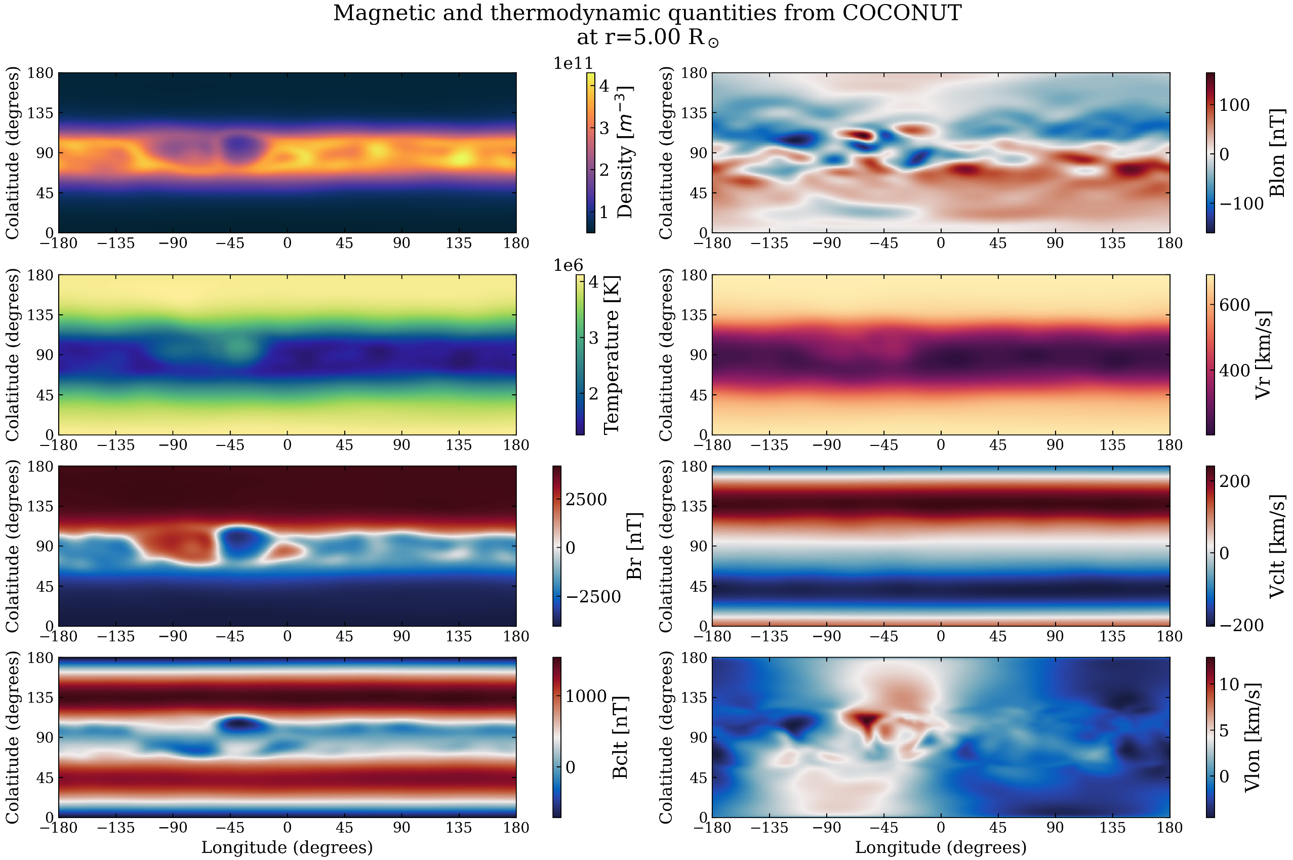
Example of 2D surface maps generated from CFmesh data.

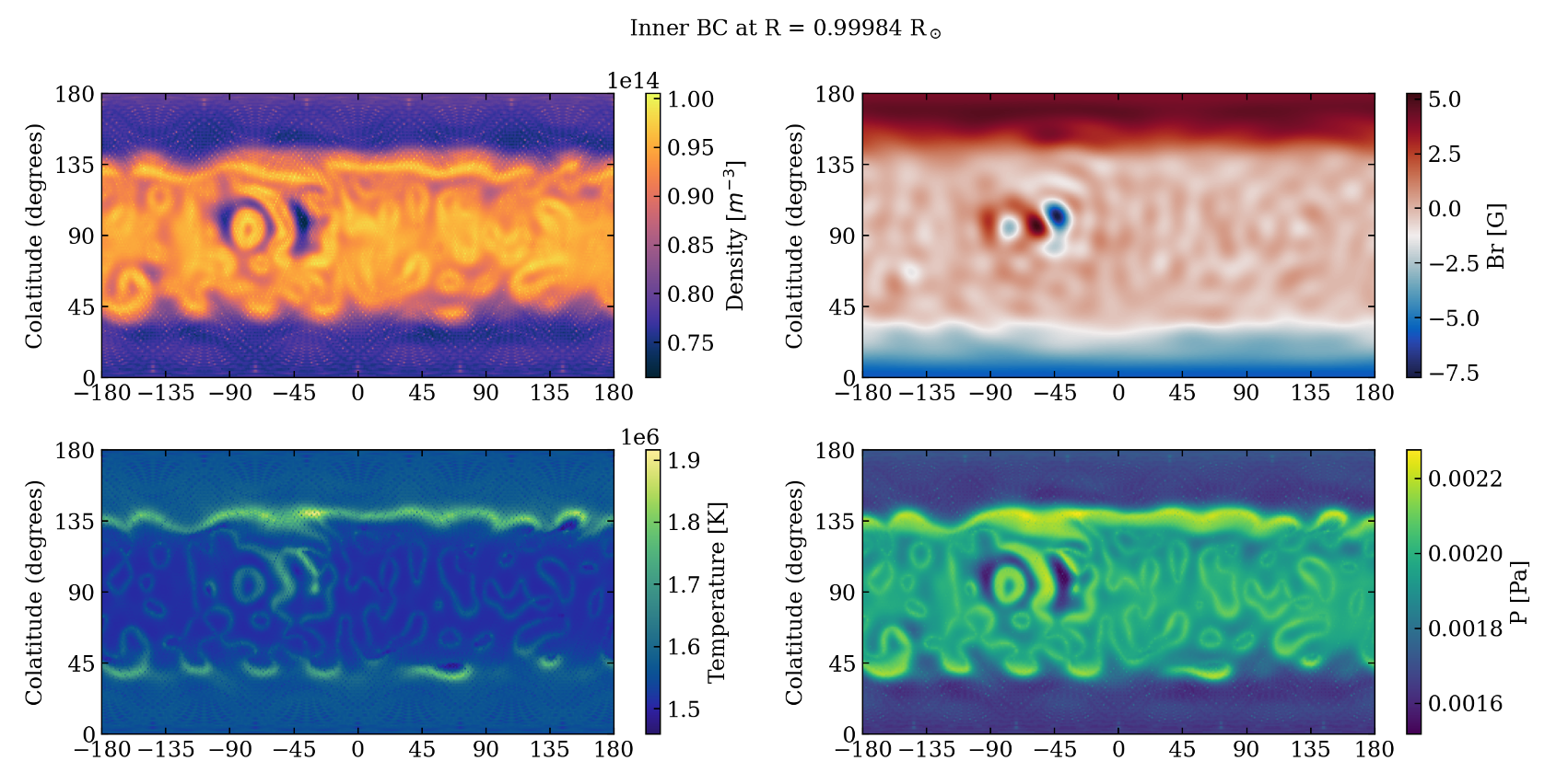
Boundary Condition Diagnostics

Two diagnostic tools are available:

• inner_bc_check

• outer_bc_check

They evaluate physical consistency of the simulation.

Inner boundary plots include:

• density

• temperature

• radial magnetic field

• pressure

Outer boundary plots include:

• sound speed

• Alfvén speed

• Mach number

• Alfvénic Mach number

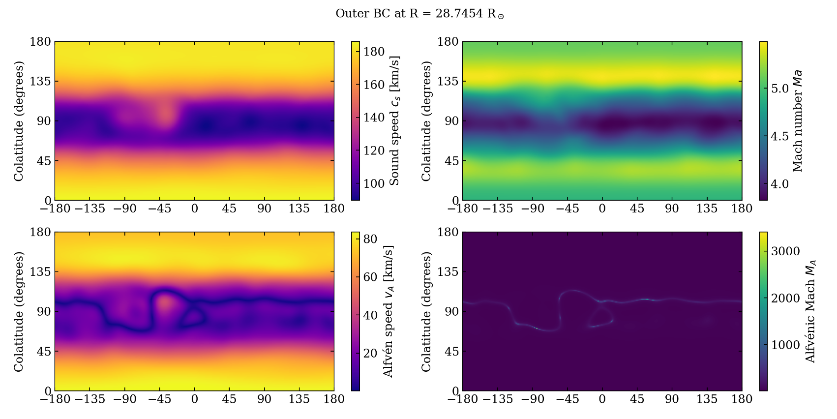
Inner and outer boundary diagnostics.

PyVista Visualization

The module uses PyVista to visualize VTU data.

Pipeline:

1. Read mesh

2. Convert units

3. Convert to spherical coordinates

4. Generate slices or 3D views

Example slice:

rc.run_coconut_reader(
    vtu_relpath="vtu/corona-mhd_0000.vtu"
)

Example PyVista slice visualization.

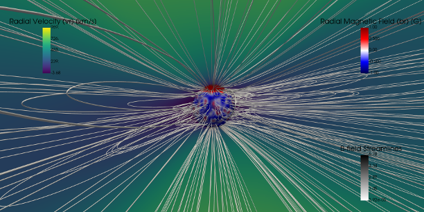
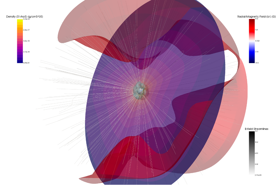
Alfvén Surface Visualization

Enable with:

rc.run_coconut_reader(..., AlfvSurf=True)

This produces:

• density slice

• Alfvén surface

• optional iso-contours

Alfvén surface visualization.

Quick Visualization Tools

Quick_Vr_Viewer

Provides a fast 2D disk visualization (Tecplot-like).

rc.Quick_Vr_Viewer(
    vtu_relpath="vtu/corona-mhd_0000.vtu",
    plane="y",
    cam_dist=150.
)

Features:

• selectable plane (x, y, z, or longitude)

• field selection (e.g. vr, br, density)

• optional magnetic field lines

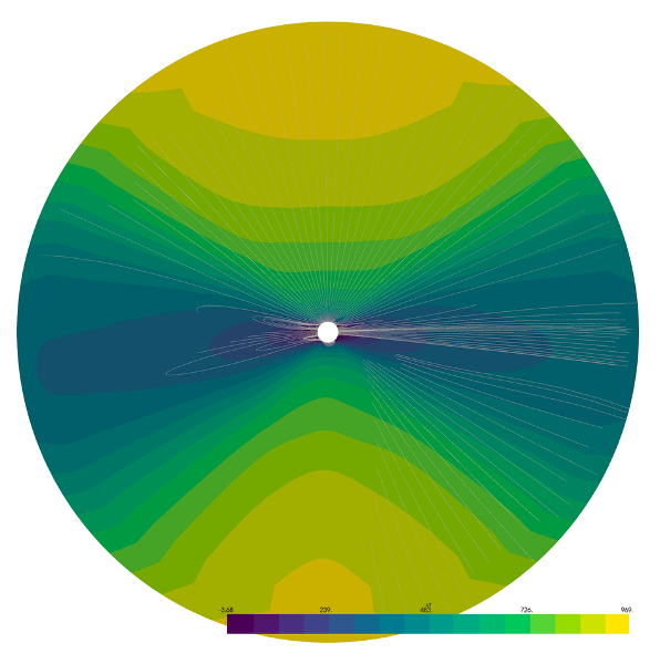
Example of Quick_Vr_Viewer output.

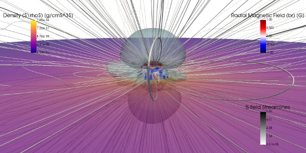
Quick_Ra_viewer

Produces a fast 3D visualization including:

• density slices

• magnetic topology

• Alfvén surface

• iso-contours of velocity

rc.Quick_Ra_viewer(
    vtu_relpath="vtu/corona-mhd_0000.vtu",
    volumic_vr=500.
)

Example 3D visualization.

Spherical Surface Visualization

Plot scalar quantities on a spherical surface at a given radius.

rc.visualize_spherical_surface_from_vtu(
    vtu_path="vtu/corona-mhd_0000.vtu",
    r_surf=2.5,
    field="vr",
    view="iso"
)

Options:

• camera view (x, y, z, iso)

• Carrington grid overlay

• customizable resolution

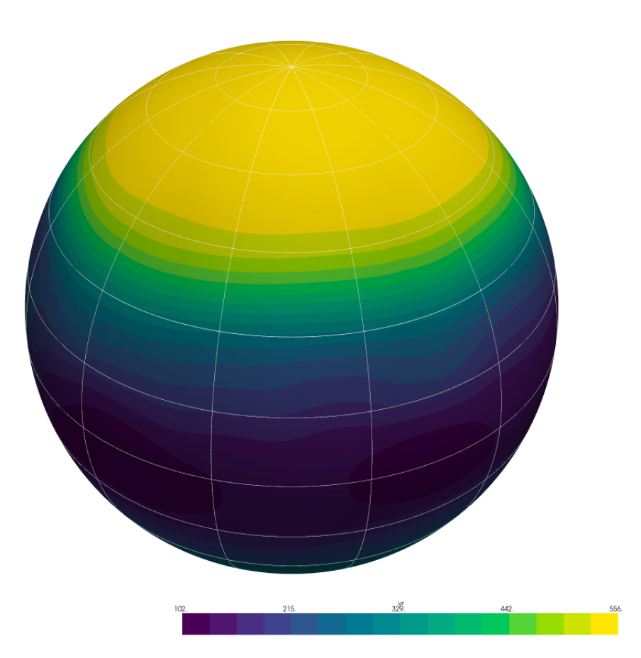
Spherical surface visualization.

Y-plane Disk Visualization

Function:

rc.visualize_yplane_disk(mesh, field="vr")

Features:

• full-disk projection

• field line tracing

• customizable seeding and integration

This provides a centered disk view similar to solar observations.

Data Flow Summary

The processing workflow is:

CFmesh  --->  .dat files  --->  2D surface plots
   |
   +---> VTU ---> PyVista ---> 2D/3D visualizations

Documentation and Help

Each function is documented via docstrings.

In IPython:

rc.run_coconut_reader?
rc.Quick_Vr_Viewer?

Source code documentation is available in:

coconut_tools/src/coconut-tools/*.py

contact: Q. Noraz